acquiring and exploring eBird data
I took up birding during a summer I spent at St. Olaf College working in
a lab that did electrophysiological experiments on the retinas of
snapping turtles. Hours in a dark room waiting for light-stimuli
experiments to run were magnitudes more interesting when I was working
through Frank Gill’s Ornithology or thinking about the birds I’d see
during my walks to and from the science building. I became acquainted
with eBird then as a tool to keep track of the birds I’d seen. For those
not in the know, eBird is a Cornell Lab of Ornithology Citizen Science
project where birders all across the world log their birding trips, what
birds they see, and where they saw them.
Fast forward 4 years and I discover you can just get eBird data??!! All of it??!! With all the data analysis and machine learning tools I’d built up over the years this seemed like a prime opportunity to combine my technical skills with something I really enjoy. This and the next few posts will document my exploration of the eBird dataset. I will focus on the specific example of one of my favorite birds, the White-Breasted Nuthatch (Sitta Carolinesis), in my home state of Minnesota.
My initial excitement to access all the data was muted when I learned the whole dataset comprises 600 million birding checklists and hundreds of GBs of data. Luckily the talented people at the Cornell Lab have built a handy R package called auk (based off the bird and the command line tool awk) to efficiently filter the data.
I heavily referenced the online guide: eBird Best Practices in my exploration. It is very well written and an extremely good guide to get started using eBird data. I start by importing libraries.
library(auk)
library(lubridate)
library(sf)
library(gridExtra)
library(tidyverse)
library(here)
library(knitr)
library(kableExtra)
However, the very first thing I had to do was use my eBird account to download the eBird dataset. As I knew I was going to focus on Minnesota, I downloaded a smaller version of the complete dataset, restricted to checklists in Minnesota. The total unzipped file size was around 17Gb - much more manageable!
Whittling the data down
As mentioned above, I will use the auk library to filter the dataset down into something manageable and workable.
# setup data directory
if (!dir.exists(here("data"))) {
  dir.create(here("data"))
}

species <- "White-breasted Nuthatch"
region <- "US-MN"

# Note - I previously pointed auk to where I keep my data
ebd <- auk_ebd("ebd_US-MN_relAug-2021.txt",
               file_sampling = "ebd_sampling_relAug-2021.txt")

# Construct filters
ebd_filters <- ebd %>%
  auk_species("White-breasted Nuthatch") %>%
  auk_state("US-MN") %>%
  auk_protocol(protocol = c("Stationary", "Traveling")) %>%
  auk_complete()

# output files


ebird_file_out <- here("data", "ebd_nuthatch_yearround_mn.txt")
sampling_file_out <- here("data", "ebd_checklists_yearround_mn.txt")

# Perform the actual filtering if the files do not already exist.
if (!file.exists(ebird_file_out)) {
  auk_filter(ebd_filters, file = ebird_file_out, file_sampling = sampling_file_out)
}
With the filtering complete I was left with two files - one ~180MB file containing all the sampling data in MN (think metadata of the checklists, one row per checklist), and one ~73.2MB file containing all the observation data in MN (the actual bird sightings, one row per bird sighting). I use the auk_zerofill function to combine these two files into one dataframe that contains all the information about the checklists and which checklists include the Nuthatch. The Best Practices eBook also suggests applying some filters to the “effort” variables to obtain more realistic ecological predictions - so I restrict the data to only include checklists that took less than 5 hours, traveled less than 5km, and included less than 10 observers.
ebird_zerofill <- auk_zerofill(ebird_file_out, sampling_file_out, collapse = TRUE)

# function to convert time observation to hours since midnight
time_to_decimal <- function(x) {
  x <- hms(x, quiet = TRUE)
  hour(x) + minute(x) / 60 + second(x) / 3600
}

# clean up variables
ebird_zerofill <- ebird_zerofill %>%
  mutate(
    observation_count = if_else(observation_count == "X", NA_character_, observation_count),
    observation_count = as.integer(observation_count),
    effort_distance_km = if_else(protocol_type != "Traveling", 0, effort_distance_km),
    time_observations_started = time_to_decimal(time_observations_started),
    year = year(observation_date),
    day_of_year = yday(observation_date)
  )

ebird_zerofill_filtered <- ebird_zerofill %>%
  filter(duration_minutes <= 5 * 60,
         effort_distance_km <= 5,
         year >= 2010,
         number_observers <= 10)

nuthatch_mn_data <- ebird_zerofill_filtered %>%
  dplyr::select(checklist_id, observer_id, sampling_event_identifier,
                bcr_code,
                county,
                scientific_name,
                observation_count, species_observed,
                state_code, locality_id, latitude, longitude,
                protocol_type, all_species_reported,
                observation_date, year, day_of_year,
                time_observations_started,
                duration_minutes, effort_distance_km,
                number_observers)

write_csv(nuthatch_mn_data, here("data","ebd_whbrnuthatch_yearround_mn_zf.csv"), na = "")
The filtering removed about 110,000 checklists out of the 680,000 total. Now the data is encapsulated in a nice tidy dataframe, and we can start to explore the characteristics of the data.
Exploring the data
First question, how many checklists sighted the White-Breasted Nuthatch?
nuthatch_mn_data %>%
  group_by(species_observed) %>%
  summarize(Total = n(), Percentage = round(n()/nrow(nuthatch_mn_data)*100, 2)) %>%
  rename("Species Observed" = species_observed) %>%
  kable()
| Species Observed | Total | Percentage |
|---|---|---|
| FALSE | 406573 | 71.46 |
| TRUE | 162412 | 28.54 |
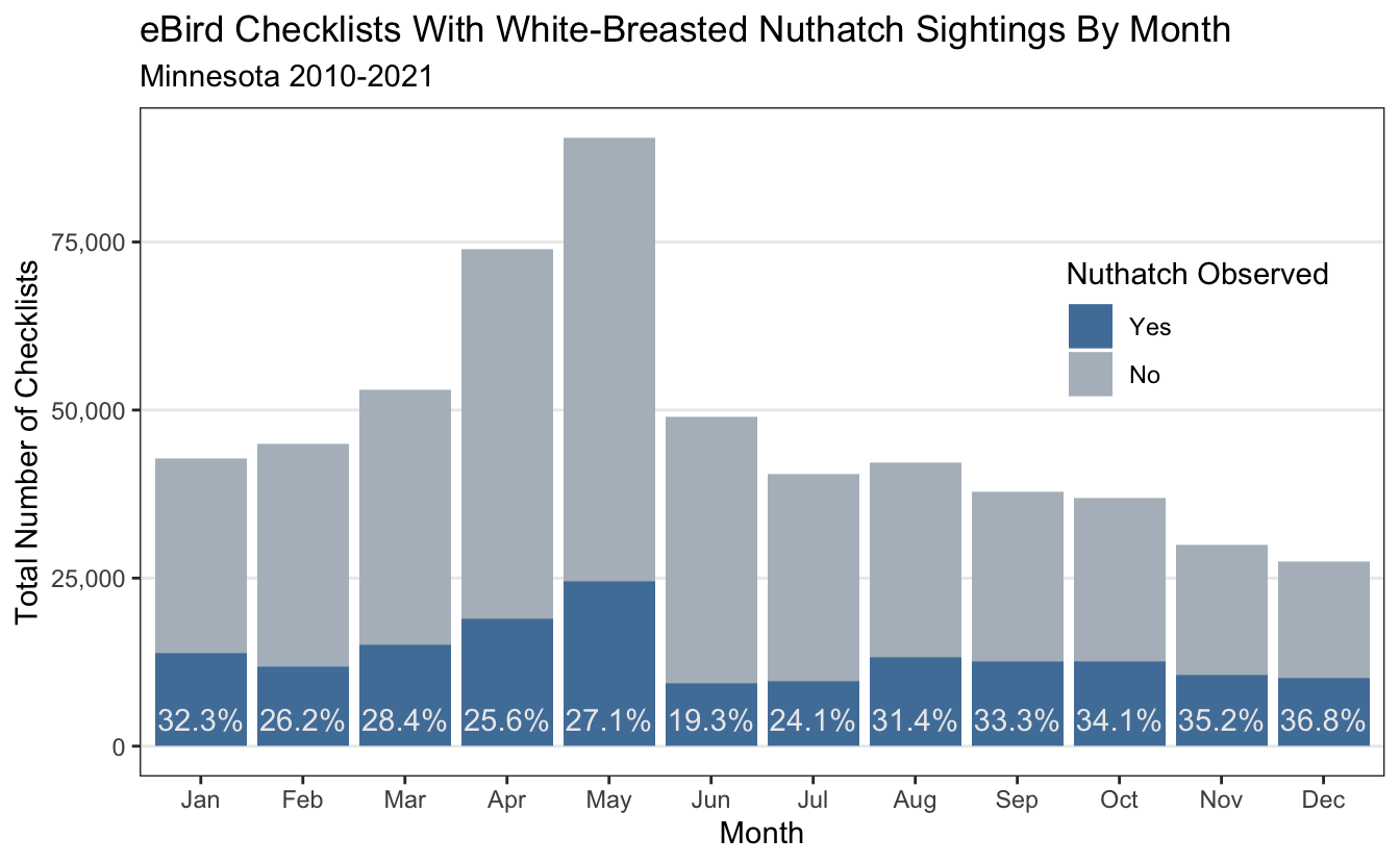
Overall about 3 in 10 checklists include a Nuthatch (when I refer to Nuthatch in this post, I always mean the White-Breasted variety). What if we also group by month?

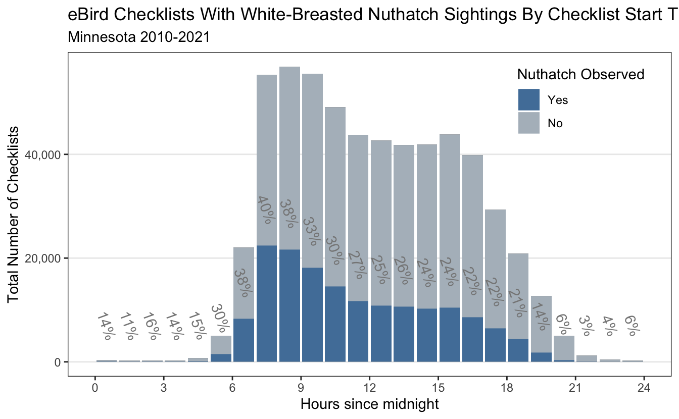
Anecdotally - It is easier to see the White-Breasted Nuthatch when the trees have lost their foliage, so I am not surprised that checklists in the fall and winter months have the highest percentage of Nuthatch sightings. Nuthatches tend to scamper up and down trees looking for food, and in face their feet are designed to support them upside down and right-side up. We can also visualize the number of checklists and sightings by the time of day (birders are morning people). This example was also done in eBird Best Practices.
# summarize data by hourly bins
breaks <- 0:24
labels <- breaks[-length(breaks)] + diff(breaks) / 2

nuthatch_mn_data %>%
  mutate(tod_bins = cut(time_observations_started,
                        breaks = breaks,
                        labels = labels,
                        include.lowest = TRUE),
         tod_bins = as.numeric(as.character(tod_bins))) %>%
  group_by(tod_bins) %>%
  summarise(n_checklists = n(),
            n_detected = sum(species_observed),
            det_freq = round(mean(species_observed)*100,0)) %>%
  ggplot() +
    geom_col(mapping = aes(x = tod_bins, y = n_checklists)) +
    geom_col(mapping = aes(x=tod_bins, y=n_checklists, fill = "#b2bcc5")) +
    geom_col(mapping = aes(x=tod_bins, y=n_detected, fill = "#517fa8")) +
    geom_text(mapping = aes(x=tod_bins, y=n_detected + 7000, label = paste(as.character(det_freq),"%", sep = "")), colour = "#878787", angle = 290) +
    scale_fill_identity(name = "Nuthatch Observed",
                        labels = c("Yes", "No"),
                        guide = "legend") +
    labs(title = "eBird Checklists With White-Breasted Nuthatch Sightings By Checklist Start Time",
         subtitle = "Minnesota 2010-2021",
         y = "Total Number of Checklists",
         x = "Hours since midnight",) +
    theme_bw() +
    theme(legend.position = c(0.85, 0.85),
        legend.background = element_blank(),
        panel.grid.minor = element_blank(),
        panel.grid.major.x = element_blank()) +
    scale_x_continuous(breaks = seq(0, 24, by = 3), limits = c(0, 24)) +
    scale_y_continuous(labels = scales::comma)

As was anticipated - most of the checklists are in the morning with a co-observed increase in the detection frequency of the white breasted nuthatch.
Mapping Checklists and Sightings
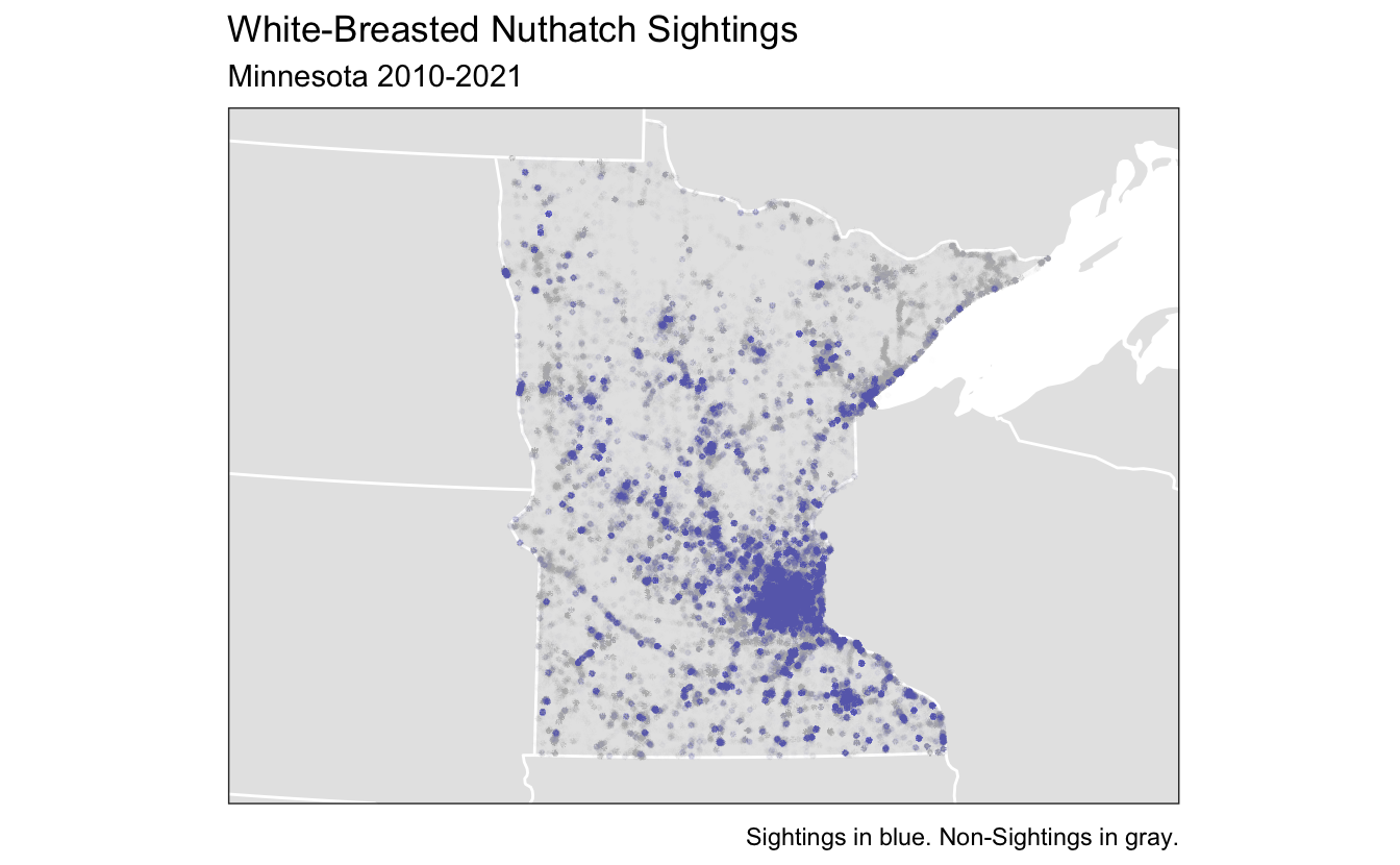
We can also plot the sightings on a map - since each checklist is associated with a latitude and longitude. I was almost able to use the script provided in eBird Best Practices, but instead of acquiring BCR data, I downloaded a shape file from the State of Minnesota to use. That data is loaded here.
map_proj <- st_crs("ESRI:102003")
ne_land <- read_sf("data/gis-data.gpkg", "ne_land") %>%
  st_transform(crs = map_proj) %>%
  st_geometry()

mn <- read_sf(here("data", "gis-data.gpkg"), "mn") %>%
  st_transform(crs = map_proj) %>%
  st_geometry()

ne_country_lines <- read_sf("data/gis-data.gpkg", "ne_country_lines") %>%
  st_transform(crs = map_proj) %>%
  st_geometry()
ne_state_lines <- read_sf("data/gis-data.gpkg", "ne_state_lines") %>%
  st_transform(crs = map_proj) %>%
  st_geometry()
I also had the goal of using ggplot for all of the figures in this - the eBird Best Practices uses plot() and par() for a lot of the maps. The biggest hurdle was setting the field of view. I found and incorporated some of the code from the very helpful blog post Here.
get_display_window <- function(lat, long, zoom) {
  zoom_to <- c(lat, long)
  zoom_level <- 5

  # Lambert azimuthal equal-area projection around center of interest
  target_crs <- sprintf('+proj=laea +lon_0=%f +lat_0=%f',
                        zoom_to[1], zoom_to[2])

  C <- 40075016.686   # ~ circumference of Earth in meters
  x_span <- C / 2^(zoom_level+0.5)
  y_span <- C / 2^(zoom_level+0.95)

  zoom_to_xy <- st_transform(st_sfc(st_point(zoom_to), crs = 4326),
                             crs = target_crs)

  disp_window <- st_sfc(
      st_point(st_coordinates(zoom_to_xy - c(x_span / 2, y_span / 2))),
      st_point(st_coordinates(zoom_to_xy + c(x_span / 2, y_span / 2))),
      crs = target_crs
  )
  window_crs <- list(window = disp_window, crs = target_crs)
  return(window_crs)
}

window_crs <- get_display_window(-94.3114, 46.278594, 5)
And then all that is left is to generate the plot itself:
nuthatch_mn_data %>%
  dplyr::select(latitude, longitude, species_observed) %>%
  st_as_sf(coords = c("longitude", "latitude"), crs = 4326) %>%
  st_transform(crs = map_proj) %>%
  ggplot(data = .) +
  geom_sf(data = ne_land, color = "white") +
  geom_sf(data = ne_country_lines, color = "white") +
  geom_sf(data = ne_state_lines, color = "white") +
  geom_sf( aes(col=species_observed), alpha = 0.01, size = 0.5) +
  scale_color_manual(values=c("#b2bcc5", "#517fa8")) +
  coord_sf(xlim = st_coordinates(window_crs$window)[,'X'],
           ylim = st_coordinates(window_crs$window)[,'Y'],
           crs = window_crs$crs, datum = window_crs$crs) +
  theme_bw() +
  labs(title = "White-Breasted Nuthatch Sightings",
       subtitle = "Minnesota 2010-2021",
       caption = "Sightings in blue. Non-Sightings in gray.") +
  theme(panel.background = element_blank(),
        axis.text = element_blank(),
        axis.ticks = element_blank(),
        panel.grid = element_blank(),
        legend.position = "none"
        )

What you should appreciate from this plot is that the majority of bird sightings are where people live, for MN this means the Twin Cities, Duluth, and Rochester mostly. This should make sense, places close to home are the most convenient to go birding at. However, this introduces some spatial bias which will have to be corrected for when I model the encounter rate later. One thing that would be interesting is to repeat this analysis for a rarer bird like the Great Grey Owl which only really appears in the far north, where the density of checklists is low.
Final Thoughts
Of course, this is only the tip of the iceberg of what can be done with
eBird data. The Best Practices eBook I have been referencing goes on to
combine this data with land cover data to model encounter rate,
occupancy, and relative abundance (for the Wood Thrush in the South and
Southeast) and that is likely what I will do next. All the code from
this post and the future posts on eBird data can be found on GitHub at
this Link.
Note: I grabbed some pixel colors from a picture of the White Breasted Nuthatch as the color scheme for the plots in this post.